Bayesian linear regression and Metropolis-Hastings sampler
on Python
Model definition
NOTE:
Theoretical considerations are mainly taken from
Let’s consider a set of observations \(\mathbf{x}\) together with observations of the target variable \(t\).
Assume that our target variable \(t\) is given by a deterministic function \(y(\mathbf{x}, \mathbf{w})\) with additive Gaussian noise:
\[\begin{equation} t = y(\mathbf{x}, \mathbf{w}) + \epsilon, \label{model} \end{equation}\]where \(\epsilon\) defines a random Gaussian noise with a zero mean and precision equal \(\beta\) (inverse variance).
The function \(y(\mathbf{x}, \mathbf{w})\) defines our model as x is a data and w is a parameters vector.
\begin{equation} y(\mathbf{x}, \mathbf{w}) = \mathbf{w}^T \mathbf{\phi}(\mathbf{x}), \label{basfunc} \end{equation}
where \(\mathbf{\phi}(\mathbf{x})\) is a set of basis functions with a dummy zero component \(\phi_0(\mathbf{x}) = 1\). These functions can belong to different families(for example Gaussian or sigmoid functions), but in all that cases the model will be called linear regression as it will be linear for \(\mathbf{w}\). The simplest choice of basis functions where \(y(\mathbf{x}, \mathbf{w}) = \mathbf{w}^T \mathbf{x}\).
So we can write
\[\begin{equation} p (t \mid \mathbf{x}, \mathbf{w}, \beta) = N(t \mid \mathbf{w}^T \mathbf{\phi}(\mathbf{x}), \beta^{-1}) \label{norm} \end{equation}\]Assuming that data points are independent and generated from (\ref{norm}), we can write a likelihood function as a function from \(\mathbf{w}\):
\begin{equation} p (\mathbf{t} \mid \mathbf{X}, \mathbf{w}, \beta) = \prod_{i=1}^N N(t_i \mid \mathbf{w}^T \mathbf{\phi}(\mathbf{x}_i), \beta^{-1}), \label{likelihood} \end{equation}
where \(\mathbf{X}\) is a vector of inputs \((\mathbf{x}_1, \mathbf{x}_2,...,\mathbf{x}_N)\) and \(\mathbf{t}\) is a vector of target points \(\mathbf{t} = (t_1, t_2,..., t_N)\) and \(\beta\) - a precision parameter.
Maximizing a log of likelihood (\ref{likelihood}) with respect to \(\mathbf{w}\) one can easili obtain an expression for the fitting parameters \(\mathbf{w}\) (so-called Normal equation)
\begin{equation} \mathbf{w}_{ML} = \left(\Phi^T\Phi\right)^{-1}\Phi^T\mathbf{t}, \label{maximized1} \end{equation}
where \(\Phi _{ij} = \phi_j(\mathbf{x}_i)\)
Here we can generate some data and check the model. Let’s generate
a set of 10 observations from the linear function \(t = -3x+2+N(0,1/\beta)\) with \(\beta = 1.0\).
We wind the fitting parameters using normal equation.
Click to see the code
    import numpy as np
    import scipy
    import matplotlib.pyplot as plt

    np.random.seed(42)
    N=10
    w_orig = np.array([-3.0, 2.0]) # true values of the parameters
    x = np.random.uniform(-1, 1, N)
    beta = 1.0 # noize precision (inverse variance)
    PHI =np.vstack((x,np.ones(x.shape[0]))).T # x with additional columns with ones (\Phi matrix)
    noize = np.random.normal(0.0, scale=1.0/np.sqrt(beta), size=N)
    t = PHI@w_orig + noize # target

    w_ml = (inv(PHI.T.dot(PHI))).dot(PHI.T.dot(t)) # normal equation

    plt.scatter(x, t, marker="x", label="data")
    plt.plot(x,PHI.dot(w_ml), c="tab:green", label="normal equation")
    plt.plot(x,PHI.dot(w_orig), c="tab:red", label="true line")
    plt.xlabel("x")
    plt.ylabel("t")
    plt.legend()
    plt.show()
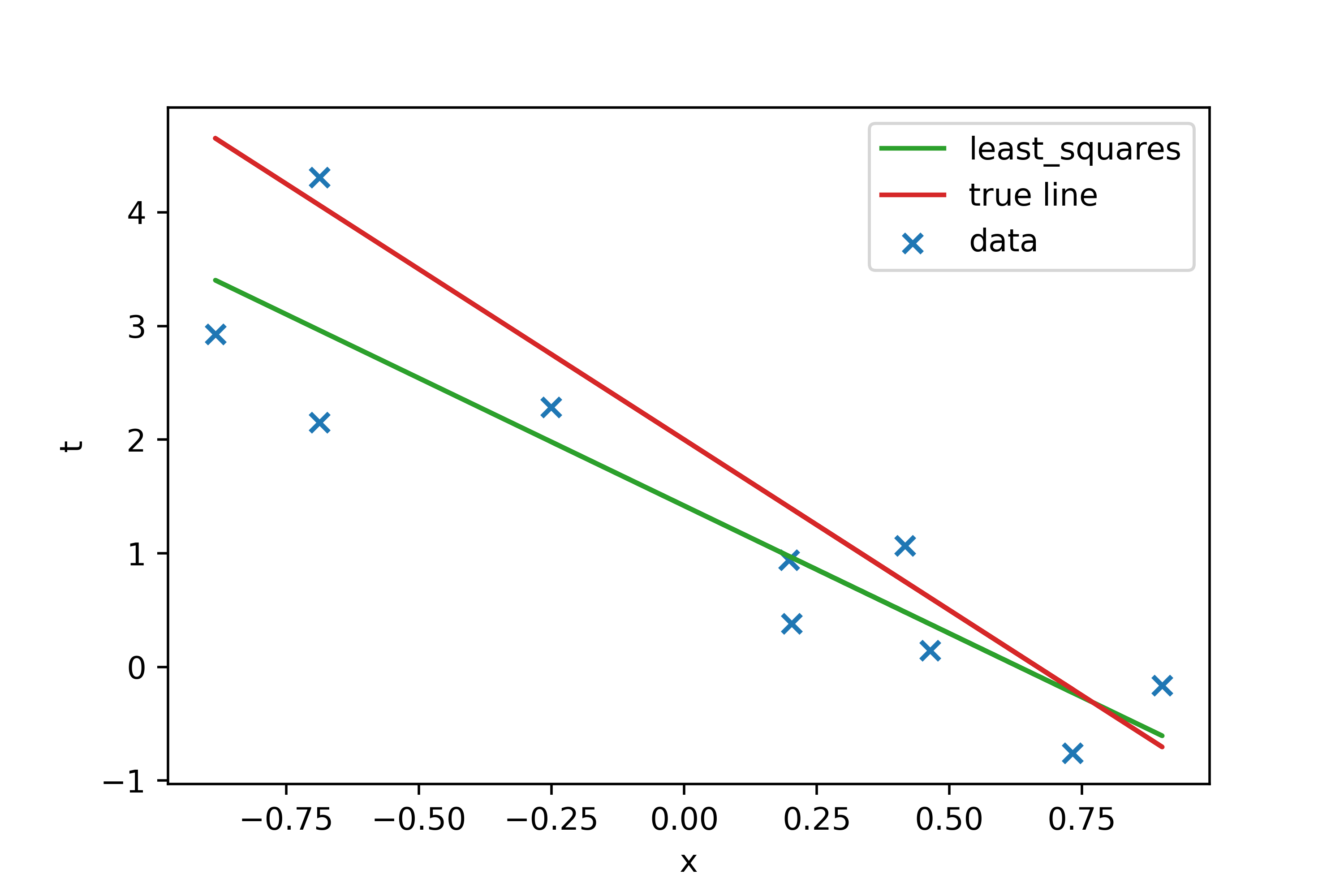
    >>> print("Original parameters:", *w_orig)
    >>> print("Normal equation parameters:", *np.round(w_ml,2))
    Original parameters: -3.0 2.0
    Normal equation parameters: -2.25 1.42
The difference with true values is \(\sim 25\%\) but this is the maximum result which can be obtained from such a dataset, so whese values could be regarded as a reference for other models.
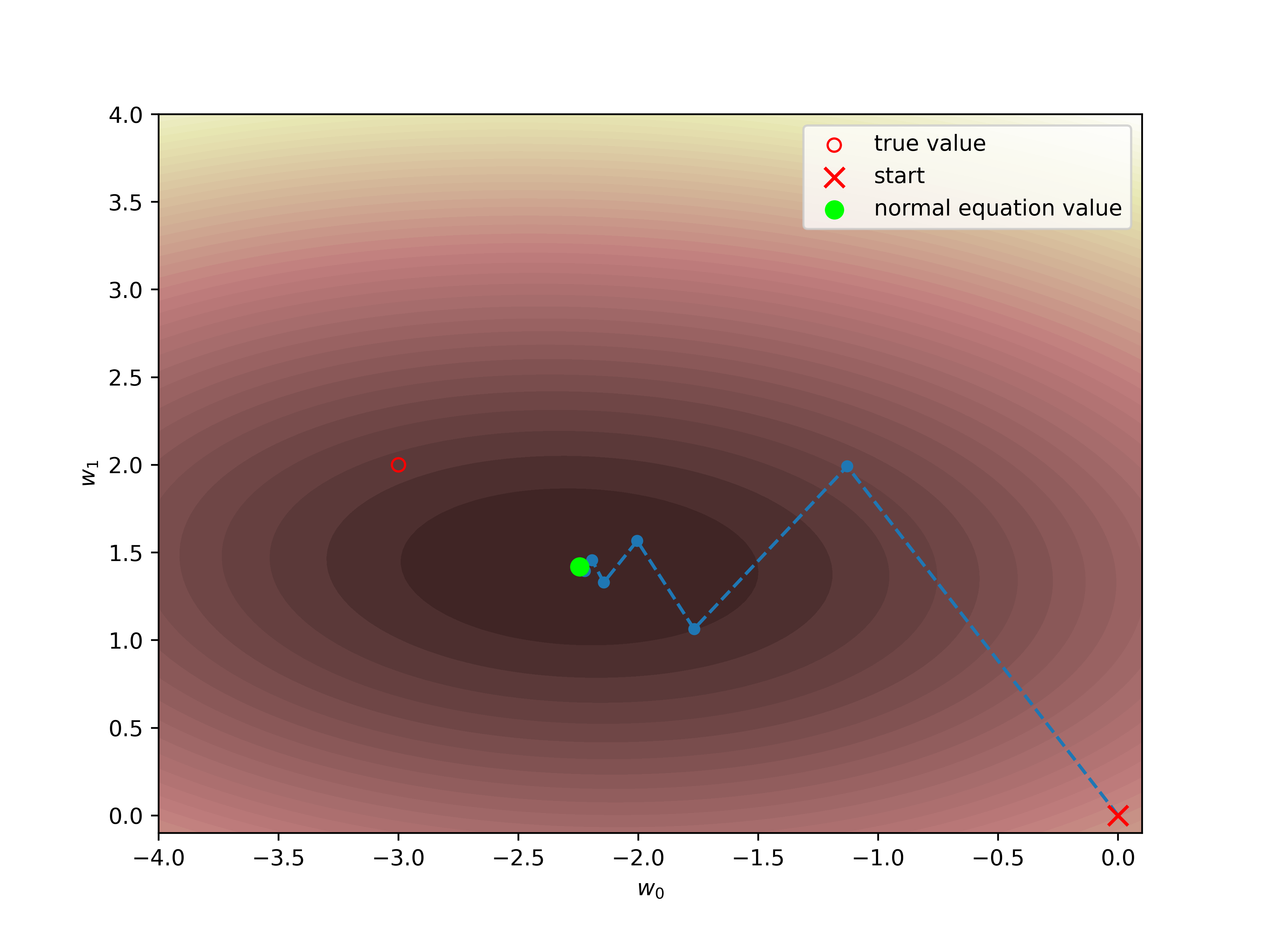
One can also apply an iterative approach,
e.g. Gradient descent. In this case, we set some zero approximation for the parameters and gradually come closer to true values. The demonstration of such a procedure is on the figure below.
Click to see the code
    w0 = np.array([0.0, 0.0])[np.newaxis,:] # first guess
    eta = 0.15 # learning rate

    xc = np.linspace(-4,0.1, 100)
    yc = np.linspace(-0.1, 4, 100)

    X, Y = np.meshgrid(xc, yc)
    www = np.moveaxis(np.stack((X,Y)), 0, -1)
    Z = np.sum((t - www.dot(PHI.T))**2, axis=-1)

    for _ in range(50):
        w0 = np.vstack((w0, w0[-1] + eta*(t-w0[-1].dot(PHI.T)).dot(PHI)))

    plt.figure(figsize=(8,6))
    plt.contourf(X, Y, Z,50, cmap='pink')
    plt.scatter(*w_orig, facecolors='none', edgecolors='r', label="true value")
    plt.scatter(w0[1:,0], w0[1:,1], s=20)
    plt.plot(w0[:,0], w0[:,1],"--")
    plt.scatter(*w0[0], label="start", marker='x', color='red', s=80)
    plt.scatter(*w_ml, facecolors='none', c='lime',s=60, label="normal equation value")
    plt.xlabel("$w_0$")
    plt.ylabel("$w_1$")
    plt.legend()
    plt.savefig("../img/linreg/descent.png", dpi=500)
    plt.show()
Bayesian approach (BA)

According to BA, we treat regression parameters not as unknown constants, but as random variables. Therefore we shall define subjective information about the set of parameters \(\mathbf{w}\) as a prior distribution. There are lots of possibilities but the simplest is to set this distribution to be a Gaussian, as it is conjugate with respect to the likelihood function (\ref{likelihood}).
\begin{equation} p(\mathbf{w}) = N(\mathbf{w} \mid \mathbf{m_0}, \mathbf{S_0}), \label{prior_w} \end{equation} where \(\mathbf{m_0}\) and \(\mathbf{S_0}\) are arbitrary defined as a first approximation.
With such a simple prior one can get the corresponding posterior distribution analytically (more details in
with well-defined parameters
\[\begin{eqnarray} \mathbf{m}_1 &=& \mathbf{S}_1\left(\mathbf{S}_0^{-1}\mathbf{m_0} + \beta \mathbf{\Phi}^T\mathbf{t}\right) \label{m1}\\ \mathbf{S}_1^{-1} &=& \mathbf{S}_0^{-1} + \beta \mathbf{\Phi}^T\mathbf{\Phi}. \label{S1} \end{eqnarray}\]According to the Bayes equation, the (\ref{posterior_w}) is nothing else but normalized product of (\ref{likelihood}) and (\ref{prior_w}). \(\mathbf{m}_1\) is a vector of means and \(\mathbf{S}_1\) is a covariance matrix for \(\mathbf{w}\).
Choosing as a first approximation \(\mathbf{m_0}=(0,0)\) and \(\mathbf{S_0} = \big(\begin{smallmatrix} 10 & 0\\ 0 & 10 \end{smallmatrix}\big)\), I obtained next results:
Click to see the code
    def likelihood(w, t, PHI, beta):
        if t.shape:
            return np.prod(scipy.stats.norm.pdf(t,loc=w.dot(PHI.T),\
                           scale=1.0/np.sqrt(beta)), axis=-1)
        else:
            return scipy.stats.norm.pdf(t,loc=w.dot(PHI.T),\
                                        scale=1.0/np.sqrt(beta))

    def m1_S1(m0, S0, y, beta, PHI):
        if y.shape:
            S1 = np.linalg.inv(np.linalg.inv(S0) + beta*PHI.T@PHI)
            m1 = S1.dot(np.linalg.inv(S0).dot(m0) + beta*PHI.T.dot(y))
        else:
            S1 = np.linalg.inv(np.linalg.inv(S0) +\
                 beta*PHI[np.newaxis].T@PHI[np.newaxis])
            m1 = S1.dot(np.linalg.inv(S0).dot(m0) + beta*PHI.T*y)
        return m1, S1

    m0 = np.array([0,0])
    S0 = np.array([[10,0],[0,10]])
    w0 = np.linspace(-5,5,100)
    w1 = np.linspace(-5,5,100)
    w=np.array([[[val0,val1] for val0 in w0] for val1 in w1])
    pr = scipy.stats.multivariate_normal.pdf(w,mean=m0, cov=S0)

    lk = likelihood(w, t, PHI, beta)
    m1, S1 = m1_S1(m0, S0, t, beta, PHI)
    pr1 = scipy.stats.multivariate_normal.pdf(w,mean=m1, cov=S1)

    plt.figure(figsize=(15,5))
    plt.subplot(131)
    plt.contourf(w0, w1, pr, cmap='RdYlGn_r')
    plt.scatter(*w_orig, marker="+", s=100, c="b", label="true value")
    plt.scatter(*w_ml, marker='x', c='black', s=50)
    plt.xlabel("$w_0$")
    plt.ylabel("$w_1$")
    plt.title("prior")
    plt.subplot(132)
    plt.contourf(w0,w1,pr1, cmap='RdYlGn_r')
    plt.scatter(*w_orig, marker='x', c='b', s=50, label="True")
    plt.scatter(*w_ml, marker='x', c='black', s=50, label="Normal equation")
    plt.legend()
    plt.title("posterior")
    plt.xlabel("$w_0$")
    plt.ylabel("$w_1$")
    plt.subplot(133)
    plt.scatter(x, t, marker='x', label='data')
    plt.plot(x,PHI.dot(m1), c="tab:green", label="label="bayesian mean")
    plt.plot(x,PHI.dot(w_orig), c="tab:red", label="true line")
    plt.legend()
    plt.xlabel("x")
    plt.ylabel("t")
    plt.xlim([-1,1])
    plt.ylim([-1,5])
    plt.tight_layout()
    plt.show()
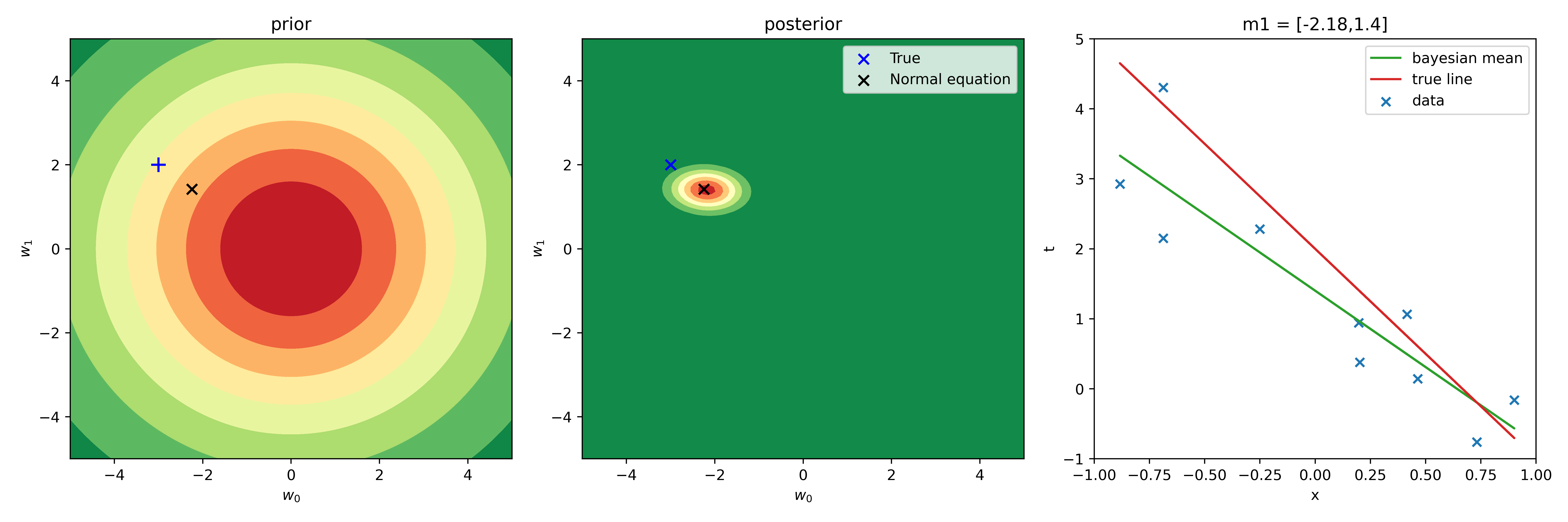
with
\[\begin{eqnarray} \mathbf{m_1} &=& (-2.18,1.4) \label{m1_res}\\ \mathbf{S_1} &=& \big(\begin{smallmatrix} 0.27 & -0.01\\ -0.01 & 0.1 \end{smallmatrix}\big). \label{S1_res} \end{eqnarray}\]The values of \(\mathbf{m_1}\) are close to the values of \(\mathbf{w}\) obtained within the frequentists’ approach (FA), but shifted towards \(\mathbf{m_0}\) values.
Metropolis-Hastings sampler for the posterior distribution
Although it was easy enough to get the posterior distribution in the previous example, it is not always the case. Metropolis-Hastings method allows to sample values from complex probability functions. As posterior is proportional to the product of the likelihood and prior, it is enough to sample from such a product to find all the neccessary distribution parameters.
The first step is to test the Metropolis-Hastings sampler on the same normal prior. We know the analytical result so we can evaluate the precision of such model.
The starting point for the sampling is chosen to be \((0,0)\), the step \(\delta = 0.5\) and the number of iterations is \(N = 10^4\). The sampling result is below.
Click to see the code
    def posterior(w, PHI, y, beta, m0, S0):
      return likelihood(w, y, PHI, beta)*prior(w, m0, S0)

    samples = np.array([0.0, 0.0])[np.newaxis]

    # for the background colormap
    w_0 = np.linspace(-6,1,100)
    w_1 = np.linspace(-1, 5 ,100)
    w=np.array([[[val0,val1] for val0 in w_0] for val1 in w_1])
    pr = prior(w, m0, S0)
    lk = likelihood(w, data_y, data_PHI, beta)

    # sampling
    while samples.shape[0] < N:
    candidate = samples[-1]+stats.uniform.rvs(loc=-delta, scale=2*delta, size=2)
    alpha = min(1, posterior(candidate, data_PHI, data_y, beta, m0, S0)\
                   /posterior(samples[-1], data_PHI, data_y, beta, m0, S0))
    u = stats.uniform.rvs()
    if u < alpha:
        samples = np.vstack((samples, candidate))

    # animation
    from celluloid import Camera

    fig = plt.figure(figsize=(8,8))
    camera = Camera(fig)
    plt.title("Posterior", fontsize=18)
    plt.xlabel("$w_0$")
    plt.ylabel("$w_1$")
    plt.xlim([-6,1])
    plt.plot(samples[:1,0], samples[:1,1],".-",
             markersize=5, alpha=0.8,
             color="deeppink", zorder=1,
             label="samples")
    plt.scatter(samples[0,0], samples[0,1],
                marker="x", s=100, c="white",
                zorder=2, label="starting point")
    plt.legend(framealpha=0.3, facecolor='bisque')
    for i in np.unique(np.geomspace(1,samples.shape[0],
                       dtype=int, num=30)):
        plt.contourf(w_0,w_1,pr*lk, cmap='RdYlGn_r')
        plt.plot(samples[:i,0], samples[:i,1],".-",
                 markersize=5, alpha=0.8,
                 color="deeppink", zorder=1,
                 label="samples")
        plt.scatter(samples[0,0], samples[0,1],
                    marker="x", s=100, c="white",
                    zorder=2, label="starting point")
        camera.snap()
    animation = camera.animate()
    animation.save(filename, fps=4, dpi=300)
Now we can find mean values of the samples and their covariance matrix.
  >>> print("Mean:", np.round(np.mean(samples, axis=0),2))
  >>> print("Covariance:\n", np.round(np.cov(samples.T),2))
    Mean: [-2.2  1.4]
    Covariance:
          [[ 0.27 -0.02]
          [-0.02  0.1 ]]
These values are quite close to analytical (\ref{m1_res}) and (\ref{S1_res}). So this method sufficiently approximates posterior probability disribution.
We can observe, that the numerical approach works, so we can define the prior in a more complicated way and numerically estimate the regression parameters.
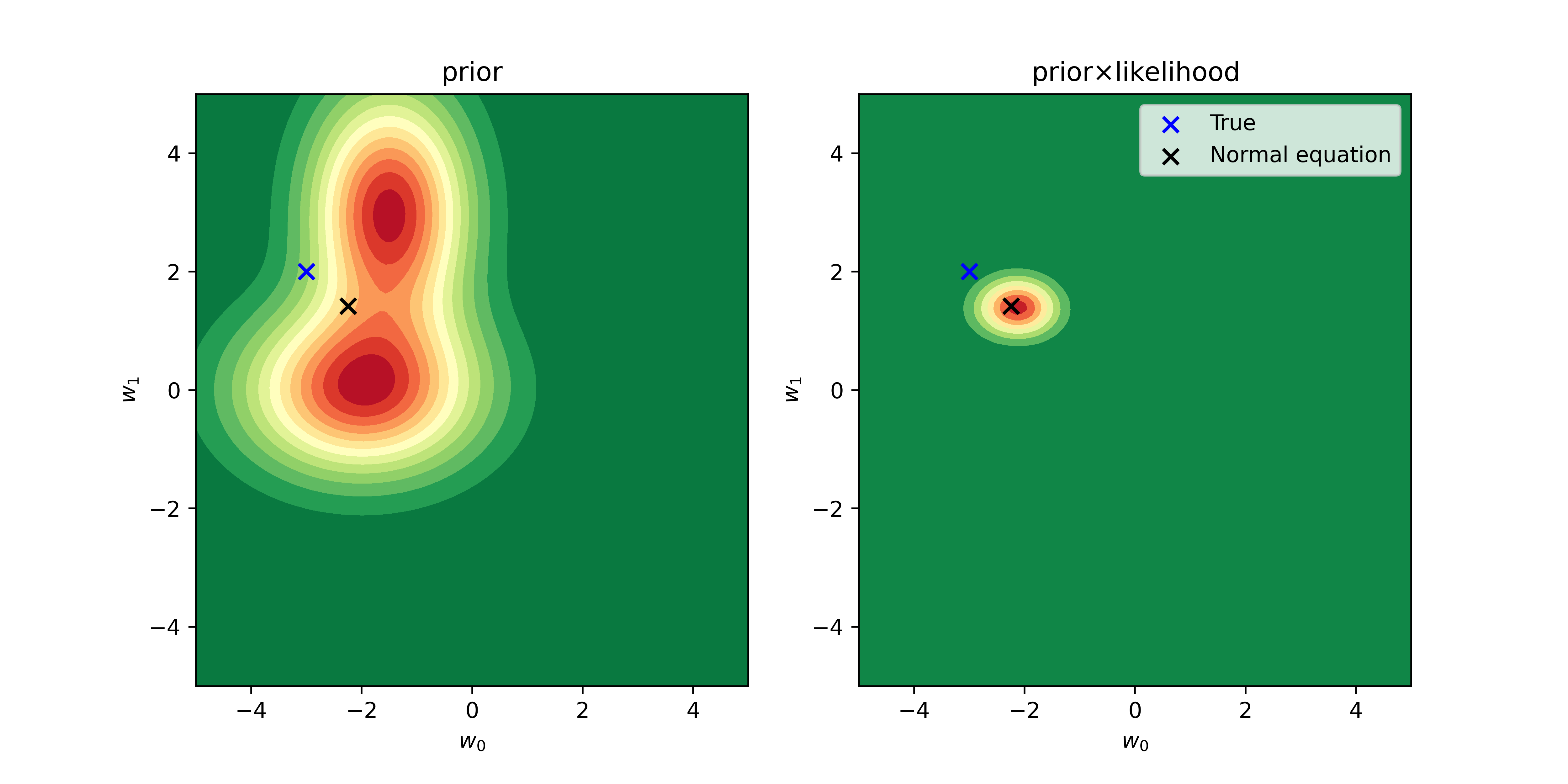
I define the prior distribution as a combiantion of two Normal distributions and apply it for the same dataset.
def prior(w):
  return 0.5*scipy.stats.multivariate_normal.pdf(w, mean=[-2, 0],
                                                 cov=[[2,0],[0, 0.9]])+\
      0.5*scipy.stats.multivariate_normal.pdf(w, mean=[-1.5, 3],
                                              cov=[[0.9,-0.0],[0.0, 1.8]])
Click to see the code
      w_0 = np.linspace(-5,5,100)
      w_1 = np.linspace(-5,5,100)
      w=np.array([[[val0,val1] for val0 in w_0] for val1 in w_1])

      lk = likelihood(w, t, PHI, beta)
      pr = prior(w)

      plt.figure(figsize=(10,5))
      plt.subplot(121)
      plt.contourf(w_0,w_1,pr, cmap='RdYlGn_r', levels=15)
      plt.scatter(*w_orig, marker='x', c='b', s=50, label="True")
      plt.scatter(*w_ml, marker='x', c='black', s=50, label="Normal equation")
      plt.title("prior")
      plt.xlabel(r"$w_0$")
      plt.ylabel(r"$w_1$")
      plt.subplot(122)
      plt.contourf(w_0,w_1,pr*lk, cmap='RdYlGn_r')
      plt.scatter(*w_orig, marker='x', c='b', s=50, label="True")
      plt.scatter(*w_ml, marker='x', c='black', s=50, label="Normal equation")
      plt.legend()
      plt.title(r"prior$\times$likelihood")
      plt.xlabel(r"$w_0$")
      plt.ylabel(r"$w_1$")
      plt.show()
Now I can generate samples using the same numerical algorythm.
  >>> print("Mean:", np.mean(samples, axis=0))
  >>> print("Covariance:\n", np.cov(samples.T))
    Mean: [-1.83022425  1.64481683]
    Covariance:
    [[ 0.62099147 -0.04302909]
    [-0.04302909  0.4241194 ]]
These values are still quite close to analytical (\ref{m1_res}) and (\ref{S1_res}). The prior I have chosen is very unrealistic, so, in fact, it only complicates the procedure. Nevertheless, the sampling method works well and makes possible to retrieve distribution parameters.
In BA we regard parameters as random variables, so we are not satisfied with only point estimations of the target variable \(t\). We would like to estimate a credible interval for our prediction as well. For the Gaussian conjugated prior it is also possible to obtain analytical solution. Still, numerical methods can be used for the predictive distribution.
I will demonstrate it in the next post.